Realtime vehicle classification for public transport by combining spatiotemporal data

I live in The Netherlands, one of the countries where almost all public transport companies publish live GPS coordinates from active vehicles. After my last article about what can be done with these coordinates, I will now describe a theoretical setup for vehicle classification taking smartphone GPS coordinates as input. The objective is to classify a vehicle, given a set of coordinates over time.

Modeling the public transport state space

Since our classification system operates in a highly dynamic environment (vehicles get delayed, take de-tours), a stateful representation of the world is necessary. State is calculated for every time $t$ and reflects the locations of all active public vehicles. We derive state from the following sources:

• General Transit Feed Specification (GTFS): static public transport schedule that is updated every 24 hours. Contains waypoints, timestamps and stops.
• Live-feed for vehicle location updates: GPS coordinates + measurement timestamps for every active vehicle with an interval between 10 and 60 seconds.

Based on the GTFS format, for each vehicle a list of spatiotemporal waypoints is created that will function as a vehicle trajectory. A trajectory describes a route over time and through two-dimensional space.

Given a time $t_{ref}$ between two waypoints $p_{i}$ and $p_{i+1}$ with timestamps $t_{i}$ and $t_{i+1}$, a possible vehicle delay (based on the live-feed) $\delta_{i}$, $\delta_{i+1}$ and GPS coordinates $(x_{i},y_{i})$, $(x_{i+1},y_{i+1})$, we get the interpolated vehicle location:

$$ x_{T}(t_{ref}) = \Big[\frac{(x_{i+1} - x_{i})(t_{ref} - (t_{i} + \delta_{i}))}{(t_{i+1} + \delta_{i+1}) - (t_{i} + \delta_{i})}\Big] + x_{i}$$

$$ y_{T}(t_{ref}) = \Big[\frac{(y_{i+1} - y_{i})(t_{ref} - (t_{i} + \delta_{i}))}{(t_{i+1} + \delta_{i+1}) - (t_{i} + \delta_{i})}\Big] + y_{i}$$

Traveller GPS location

Dependent on the implementation the interval in which traveller location is received can vary from 20 updates per minute (in a fast moving train with the implementation on the foreground) to 0 updates per minute (in an idle state, with the implementation closed).

Classification

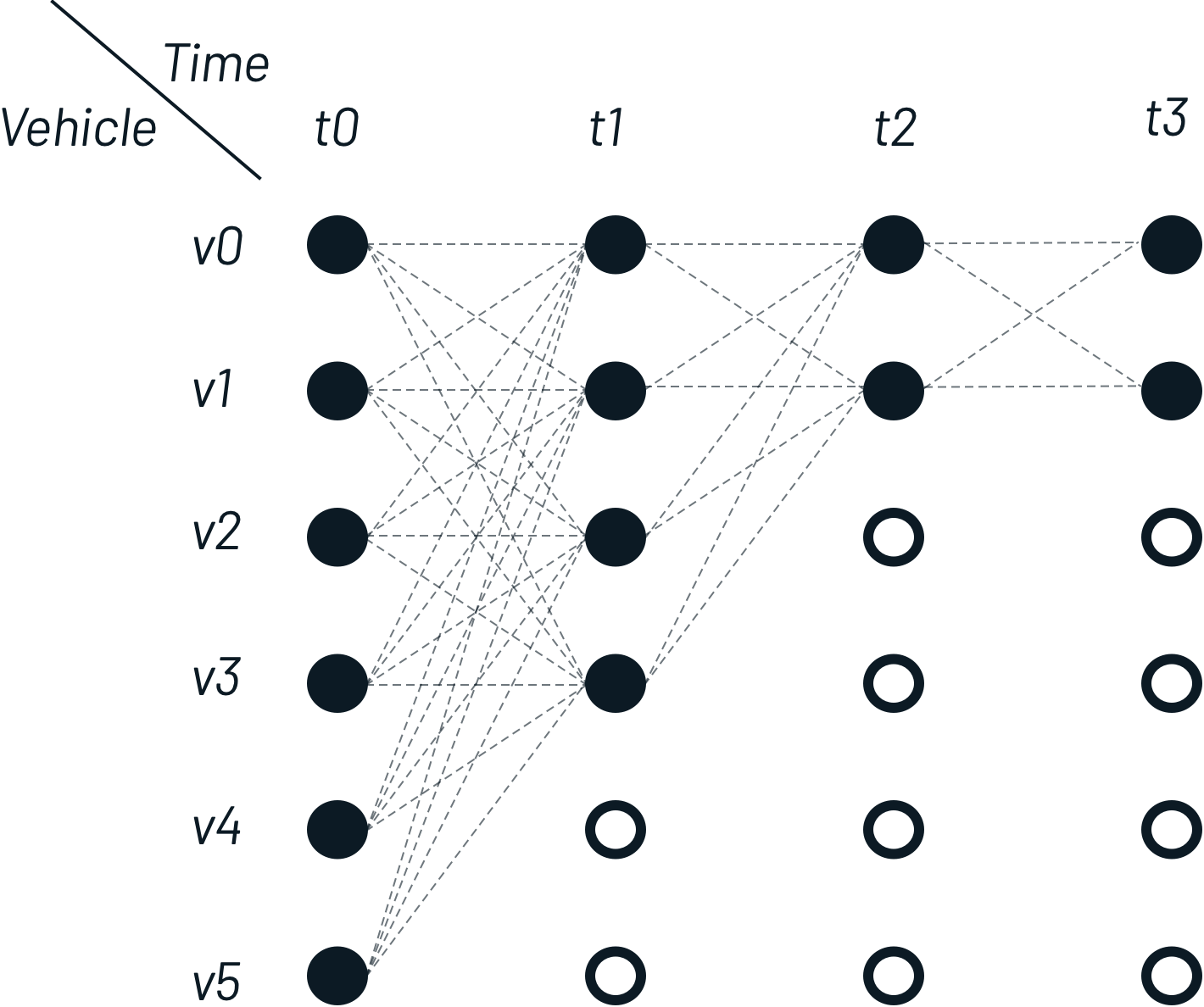
For every measured and retrieved traveler GPS location, we search in the public transport space for vehicles within radius R given measured time T. After retrieving the traveler’s location multiple times, we construct the following Hidden Markov Model in a sliding window manner:

Emission probability

Emission probability gives the likelihood that a measurement resulted from a given state, given that measurement alone. For vehicle matching, given a location measurement $z_{t}$, there is an emission probability for each vehicle $v_{i}$, $p(z_{t}|v_{i})$. This returns the likelihood that measurement $z_{t}$ would be observed if the traveller was actually in vehicle $v_{i}$. For a given $z_t$ and $v_i$, the closest position of a vehicle is denoted as $x_{t,i}$. The distance on the surface of the earth between the measurement and the vehicle candidate is $||z_{t} - x_{t,i}||_{great circle}$. Due to GPS noise (a potential tuning parameter), a correct match can differ. By taking GPS noise into account, emission probability is calculated as follows:

$$ p(z_{t}|v_{i}) = \frac{1}{\sqrt{2 \pi \sigma_{z}}} e ^{ -0.5 \left( \frac{||z_{t} - x_{t,i}||_{great circle} }{\sigma_{z}} \right) ^{2} }$$

Transition probability

Each measurement $Z_t$ has a list of possible vehicle matches, as does the next measurement $Z_{t+1}$. Transition probabilities give the probability of a traveler moving between the candidate vehicle matches at these two times. For a measurement $Z_t$ and candidate vehicle segment $V_i$, we denote the longitude/latitude point of the vehicle nearest to the measurement as $x_{t,i}$. For the next measurement $Z_{t+1}$ and candidate vehicle $v_j$, the corresponding point is $X_{t+1,j}$. The distance between those two points is computed using the GTFS route schedule and follows the planned trajectory to the closest stop on the trajectory¹. A correct pair of matched points typically results in a small ‘route distance’ to the same stop for $X_{t,i}$ and $X_{t+1,j}$. The total distance between two points is notated as $||x_{t,i} + x_{t+1,j}||_{route}$.

Work in progress

I am currently working on a technical implementation of this, which can be followed here.